Educational Research and Statistical Analysis Training for Teachers - Collection of R Practices from Sessions 13–20

Previously, I used to wonder whether I really needed to learn R when I already knew Python.

Through this training, I realized that there’s actually no need to use Python when doing research.

In Python, you’d have to do linear regression with numpy, draw graphs, calculate the p-value, and handle everything yourself, but in R you can finish it all with just lm and summary.

So today, I’m going to review all the R practice content we’ve learned so far and show some practice examples using real data.

1. Example data

The example data is a dataset of U.S. students’ test scores uploaded on Kaggle.

For those who are not signed up on Kaggle, I’ve attached a link below.

This dataset was created to examine the effects of factors such as parental background and test preparation courses on students’ academic performance.

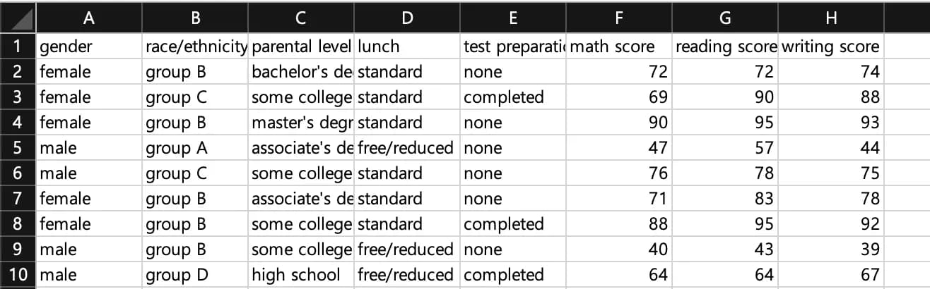
I’ve pasted the internal values of the dataset below.

To explain briefly: gender is the student’s sex, race is ethnicity, parental level is the parents’ education level, lunch is the price level of the school lunch, and test preparation indicates whether the student completed a test preparation course.

2. Opening a csv file in R Studio

The command to load a file in R Studio is read.

If you find it annoying to type the file path, you can just click the file, copy it, and then paste; the path will be inserted.

Or you can use the file.choose() command to select the file in a Windows dialog.

For reference, you can run each line of code with ctrl + enter (cmd + enter on Mac).

data <- read.csv("파일경로")
// dat <- read.csv(file.choose())

head(data)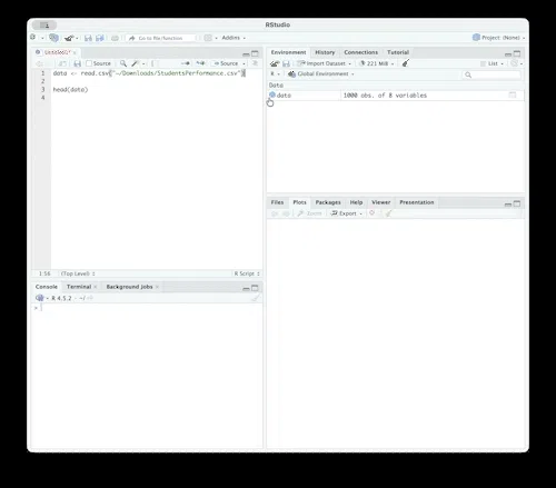

3. Linear regression analysis

Now let’s run a simple linear regression with this dataset.

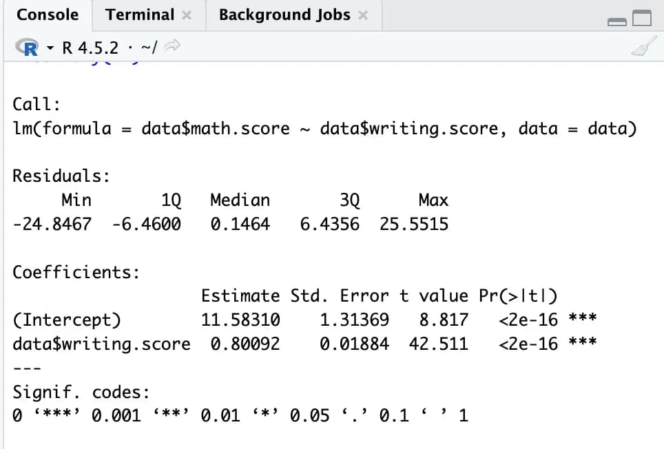
The function lm takes as its internal parameters lm(dependent_variable ~ independent_variable, dataset) in that order.

For example, if you want to look at the relationship between math scores and writing scores, you can run the following:

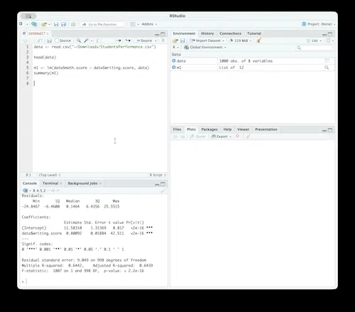
m1 <- lm(data$math.score ~ data$writing.score, data)
summary(m1)

With this, the linear regression is completed very easily.

Without setting anything else, it conveniently outputs values detailed enough for a research paper, including errors, t-test, and p-value.

4. Drawing charts

Drawing graphs is also extremely simple.

Just by typing plot(m1), R draws most of the necessary charts for you.

If you want a specific plot, you can specify the x-axis and y-axis values in order, separated by a comma.

5. Multiple regression analysis

When there are many variables, you can list all the independent variables in the lm function’s independent-variable position, separated by +.

For example, if you want to see how reading and math scores affect writing scores, you can analyze it as follows:

m2 <- lm(data$writing.score ~ data$reading.score + data$math.score, data)
summary(m2)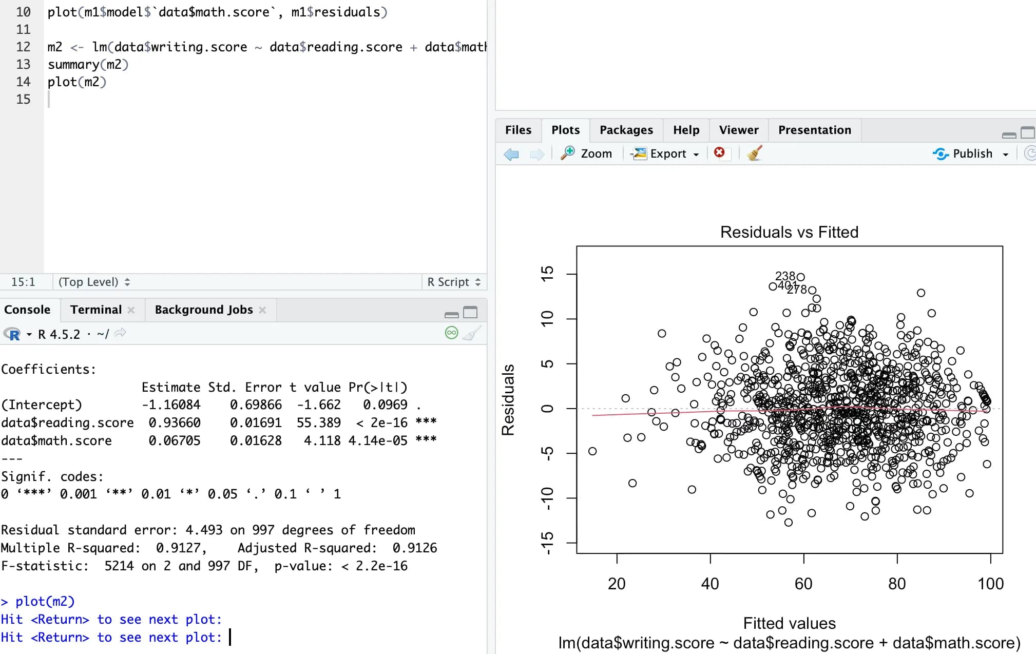

6. Handling categorical variables (non-numeric data)

Categorical variables are variables that divide data into qualitative groups or categories.

They are used to handle non-numeric data such as gender or education level.

Here, let’s use the simplest example, gender.

We will use the ifelse() function to inject a dummy variable called gender1 into data.

data$gender1 <- ifelse(data$gender == "male", 0, 1)
// 첫번째 조건이 참일경우 0, 거짓일 경우 1을 입력
head(data)

After doing this, if you check the table, you’ll see that a new gender1 column has been created, with 1 for female and 0 for male.

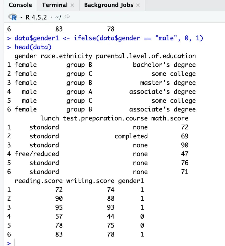
Now you can use this to run a linear regression analysis.

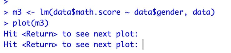
Interestingly, even if you don’t do this and just put gender in directly, the analysis still works.

m3 <- lm(data$math.score ~ data$gender, data)
plot(m3)

This is because R internally processes character-type data the way we did above and then runs the analysis.

Gender is easy because there are only two categories, but it’s a bit different for variables like parental education level or group, which have multiple categories.

If there are n categories, you need n-1 dummy variables.

You can create them manually, but it doesn’t seem like a bad idea to just entrust your soul to R.

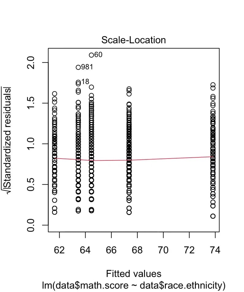
m4 <- lm(data$math.score ~ data$race.ethnicity, data)
summary(m4)
plot(m4)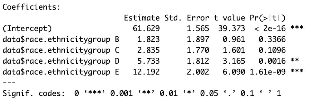

7. Calculating and using residuals with resid

Using resid, you can calculate the residuals of each term relative to the linear regression line.

By looking at the residuals, you can check whether the data is linear and what the variance looks like.

First run the analysis, then use one variable and the analysis result to calculate residuals and plot them.

m5 <- lm(data$math.score ~ data$writing.score, data)
res1 <- resid(m5)

plot(data$writing.score, res1)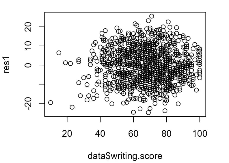

Plotting the graph like this shows that the actual data is not homoscedastic.

In this case, you need to adjust the scale for each value.

8. Interaction analysis using R - stepwise regression

Stepwise regression is a method where you add variables one by one to check their influence.

The researcher can add them manually, but R can also do it automatically.

m7 <- lm(data$math.score ~ ., data)
m8 <- step(m7, direction = "both")
summary(m8)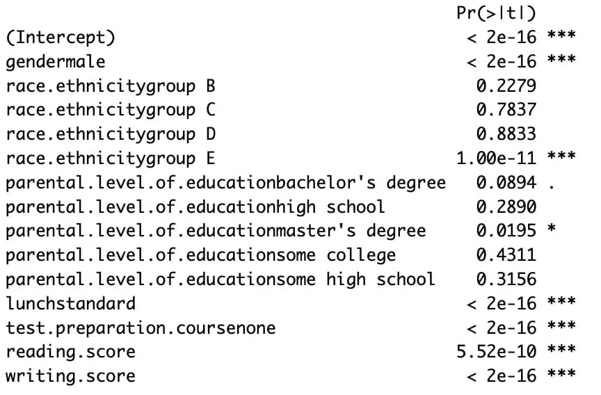

This method is easy to run, but the interpretation is tricky.

That’s why people say they prefer hierarchical regression, which analyzes according to the researcher’s intent.

9. Thoughts

I thought I could just throw everything into a stepwise regression, pick the model that explains the data best, and then draw conclusions in the direction of the lowest p-value, but that wasn’t the case.

R is convenient, but it made me realize that the researcher’s thought process is extremely important for drawing conclusions.

Before studying, I thought I could solve everything with Python without learning R, but that was a huge misjudgment.

I have come to worship R.